Homology-based Essential Gene Discovery (HEGD) Tool. [Bioinformatics].

HEGD is a computational tool that uses protein sequences of known essential genes in multiple species to predict gene essentiality in unassessed species.

Project Status: In Progress

Background.

Essential genes are genes that are thought to be necessary for the survival of an organism. All organisms share groups of essential genes involved in processess associated to DNA Replication, Transcription, Translation, and Metabolism. However, species have developed different sub-sets of essential genes throughout the span of millions of years of evolution. Essential genes are often identified throughout transposon-mediated mutagenesis studies. In these types of studies, transposons - which are mobile genetic elements - are randomly inserted in as many positions in a genome as possible, and cells that survive after a given cell culture period are sequenced. The genes of surviving cells are screened for transposon-mediated mutations: it is expected that essential genes fail to accumulate such mutations, given that cells would not tolerate them if the genes affected were truly essential.

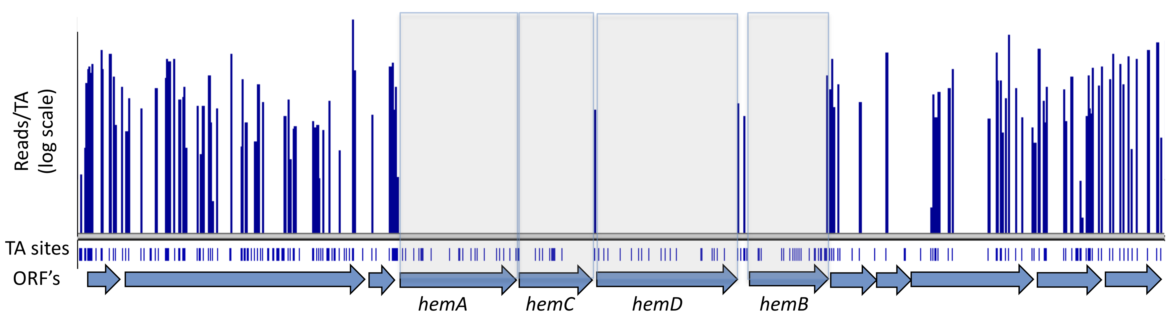
Figure 1: Identification of essential genes via genome-wide screen. Genomic regions corresponding to the genes hemA, hemC, hemD, and hemB failed to accumulate insertions of transposons - making said genes potentially essential. Source: Wikipedia

These types of studies require a lot of time an effort. Instead, we suggest implementing a homology-based machine learning model based on previous work [1] for the prediction of species-specific essential genes. This strategy assumes that essential genes are conserved amongst multiple species per kingdom, given their biological relevance.

Project.

Objective: Use the protein sequences of known essential genes in multiple species to predict essential genes in a previously unassessed species/strain.

The figure below only speaks well to trained data scientists. As a novice, you will need to continue reading this document in order to fully understand the whole approach and what your role will be in its implementation.

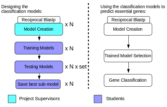
Figure 2: Concept behind HEGD. N number of models are created through reciprocal Blastp alignments between the proteins of N species with the goal of identifying orthologs - genes in different species that evolved from a common ancestral gene by speciation - of known essential genes. Models are then trained and tested using a Support Vector Machine (a type of supervised machine learning model). Multiple sub-sets of each model are generated through feature selection prior to performing cross validation. Once the models are properly trained and tested, users can then input the proteome of previously unassessed species, and a trained model is selected based on evolutionary distance - a number that defines how closely related a species is to another - with the purpose of classifying protein-coding genes as essential or non-essential. We have highlighted in Cyan the tasks that have been completed by Project Supervisors, and in Purple the tasks that will be implemented by the Students attending this course. To understand the HEGD approach in detail, please continue reading.

• Reciprocal Blastp.

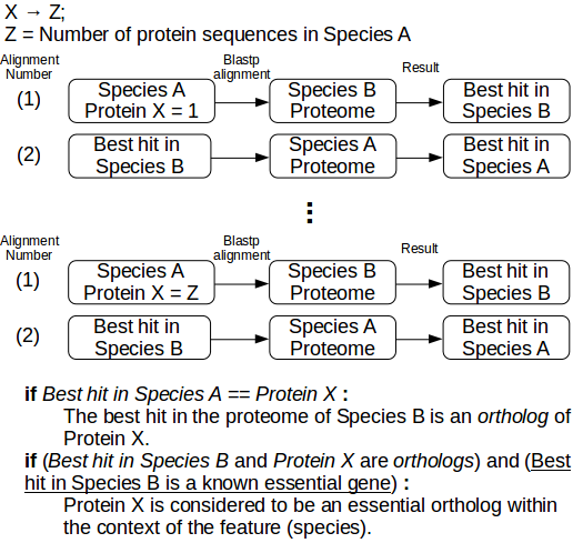
  Figure 3: Procedure for reciprocal blastp alignments. Given two species, A (Query) and B (Reference), each protein product in Species A (we will refer to each individual protein product as Protein X) is aligned with blastp to the whole proteome of Species B, and the best hit (alignment) is collected. The protein product pertaining the best hit in Species B is aligned to the whole Proteome of Species A, and the best hit is collected. If the best hit in Species A is equivalent to Protein X, then the protein hit in Species B is considered an ortholog of Protein X. By using a database of known essential genes per species, like the Database of Essential Genes (DEG), we can classify orthologs of Protein X as essential orthologs. These steps are repeated until the whole proteome of Species A is assessed. Multiple reciprocal blastp alignments are performed for every reference species (i.e. species that possess a list of experimentally determined essential genes) - see Model Creation.

Result of a single reciprocal blastp alignment (Species A < - > Species B):

Gene         Essential_Ortholog
Gene_1       1                       <-Yes
Gene_2       0                       <-No
Gene_3       0                       <-No
...
Gene_Z       1                       <-Yes

• Model creation.

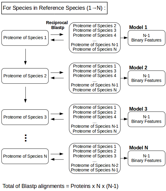
  Figure 4: Creation of a model per reference species based on multiple reciprocal blastp alignments. For every species in N Reference species, N-1 reciprocal blastp alignments are performed against the remaining Reference Species in order to identify essential orthologs. This yields datasets with N-1 Binary features, which can be used to train and test machine learning models like Support Vector Machines.

Result of multiple reciprocal blastp alignments per species model:

Model 1 (Species 1)   |     Species 2    Species 3      ...     Species N
Gene_1                |         1           0                       1
Gene_2                |         0           0                       0
...                   |        ...         ...                     ...
Gene_Z                |         1           1                       1

Model 2 (Species 2)   |     Species 1    Species 3      ...     Species N
Gene_1                |         1           1                       1
Gene_2                |         0           0                       1
...                   |        ...         ...                     ...
Gene_Z                |         1           1                       0

.
.
.

Model N (Species N)   |     Species 1    Species 2      ...      Species N-1
Gene_1                |         0           1                       1
Gene_2                |         0           0                       0
...                   |        ...         ...                     ...
Gene_Z                |         1           0                       0

Community tasks.

This section contains the theoretical knowledge pertaining tasks that each work group will be completing. All Python code involving said tasks will be discussed and implemented within bioXJMB’s Slack work group (see below).

Group 1: Evolutionary distance of two species by proteome comparison.

In order to classify genes of species that have no experimentally determined essential genes, a single trained model from the N reference models available needs to be selected. The question then remains as to which. We aim to use evolutionary distance as a metric to select for said trained model, as classification accuracy is expected to increase as evolutionary distance between species decreases.

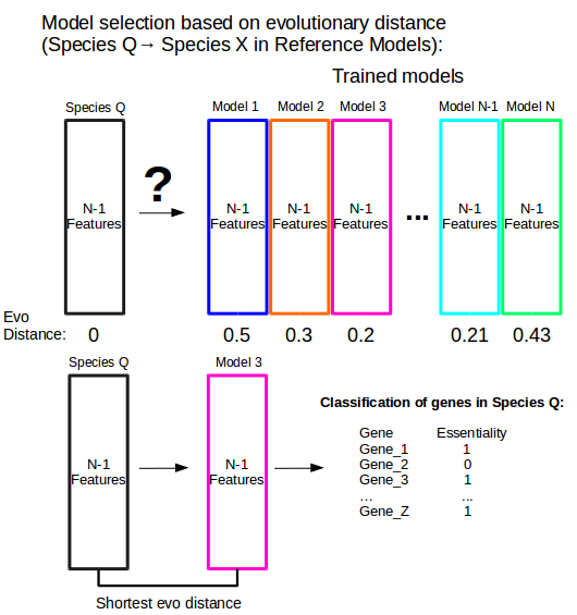
Figure 5: Model selection based on evolutionary distance. Species Q is a species that does not have a set of experimentally determined essential genes. One of the trained models from N reference models must be chosen in order to classify the genes of Species Q as essential or non-essential. The model with the shortest evolutionary distance between Species Q and each trained reference model (Model 3, in this case) is chosen.

• Calculating evolutionary distance.

  Many methods have been developed to calculate evolutionary distance, but we are only interested in implementing a computationally inexpensive way to compare the relatedness between all protein products found in two Species, A and B. To acheive this, we can treat amino acid sequences as strings of length k, or k-strings, where each protein product is constructed from multiple k-strings [2].

To explain how this notation is pertinent to estimating relatedness of the proteome of two species, consider the following:

Let k = length of k-string

Given that there are 20 amino acids found in most Earth-bound species, we can assume that there are 
20^k possible amino acid combinations for any given k-string.

Example: If k = 2, 20^k = 20^2 = 400, and so there are 400 possible amino acid combinations for any 
given k-string.
i.e.     amino acids = ["A","C","D","E","F","G","H","I", "L","K","M","N","P","Q","R","S","T","V","W","Y"]
         k-string combinations = ["AA","AC","AD","AE","AF","AG","AH","AI", "AL","AK","AM","AN","AP","AQ",
         "AR","AS","AT","AV","AW","AY", ... , "YA","YC","YD","YE","YF","YG","YH","YI", "YL","YK","YM",
         "YN","YP","YQ","YR","YS","YT","YV","YW","YY"] <- 400 amino acid combinations
         
By fragmenting individual proteins into k-strings, we can search for and report all possible amino acid 
k-string combinations within the proteome of a species. 

Let Protein X = "MYKCYK", and L = length of Protein X

There are (L - K + 1) possible k-string fragmentation patterns of length k in Protein X.
i.e. if k = 2, 
     Protein X Fragments = ["MY","YK","KC","CY","YK"] <- (L-K+1) = (6-2+1) = 5 fragmentation patterns
     
     - The frecuency of the k-string "AA" in Protein X Fragments is 0.
     - The frecuency of the k-string "YK" in Protein X Fragments is 2.

The frecuency of each possible amino acid k-string combination in the proteome of a species can be used to 
calculate probabilities of k-string occurrence. Said probabilities can be implemented in order to calculate 
k-string correlations between two species and, ultimately, evolutionary distance. 

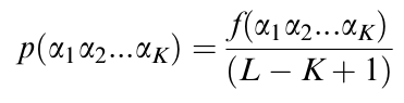
Figure 6: Probability of finding a particular k-string in a given protein sequence. The probability of finding a particular k-string (α₁α₂…α_k, where α = amino acid) in a given protein sequence - say Protein X - results from the frecuency of said k-string in Protein X, divided by the amount of possible k-string fragmentation patterns of length k in Protein X (i.e. Length of Protein X - k + 1). Each individual probability per protein can be added up to yield the probability of finding a particular k-string in ANY given protein sequence of the species in question.

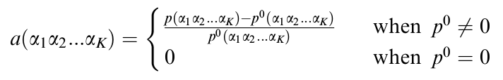
Figure 7: Emphasizing selective diversification of protein sequences. Neutral mutations (mutations that have no impact on biological fitness) lead to randomness in the k-string composition of proteins. In order to emphasize the selective diversification of sequence composition, we can subtract a random background, in the form of a predicted or inferred probability (P₀), from the probability obtained via k-string frecuency assessment.

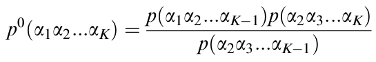
Figure 8: Predicted Markovian Probability (P⁰) of finding a particular k-string in a given protein sequence. A widely used Markov model [3] can calculate a predicted probability that accounts for the random background discussed in the description of Figure 7.

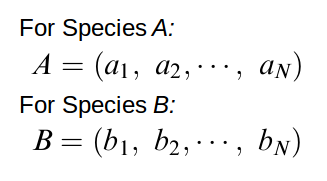
Figure 9: Representative vectors for Species A and B. Each representative vector possesses a Y-dimensional space, where Y=20^k, of composition vectors. Representative vectors A and B store Y results (i.e. one for each possible k-string) from the formula portrayed in Figure 7.

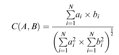
Figure 10: Correlation of Species A and B, defined by the cosine function of the angle between the two representative vectors, A & B. The correlation of Species A and B actually refers to their proteomic distance, which resides in the interval (-1,1).

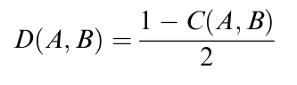
Figure 11: Normalization of correlation between Species A and Species B yields evolutionary distance. Because the cosine function defining the correlation of Species A and B results in values between -1 and 1, we can use this formula to normalize values to the interval (0,1).

Group 2: Training and testing a Support Vector Machine for the classification of genes as essential or non essential.

Support Vector Machines (SVM) are one of the most widely used machine learning approaches when it comes to Biological Data. Each data point in an SVM is viewed as a p-dimensional vector, where such points are expected to be able to linearly separate with a (p-1)-dimensional hyperplane. Such a hyperplane is referred to as the optimal hyperplane, and decision boundaries are generated with the help of support vectors - vectors that greatly contribute to the identification of an optimal hyperplane.

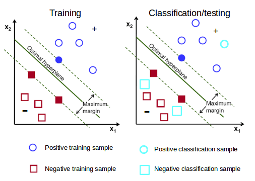
Figure 12: Training VS Classifying/Testing in a two-dimensional SVM. SVM models are first trained using a training dataset that contains two features (value columns) or more and a class label (+ or -). Each sample (row) contributes to the identification of an optimal hyperplane, which creates the decision boundaries that dictate classification results. Trained models can be tested using testing datasets that share the same features, but not the same samples. Testing sets also possess known labels. When testing trained models, each testing sample is assigned a label based on the decision boundaries established throughout training; assigned labels are compared to known labels and an accuracy score is used to rank the performance of the model. Once a satisfactory threshold is reached, trained models can be used to infer the labels of unclassified datasets.

We will train Support Vector Machines using multiple model-subsets derived from the N models created from each reference species, and we will test each model sub-set through cross-validation in order to keep the most accurate one (see Figure 13 below).

• Feature Ranking.

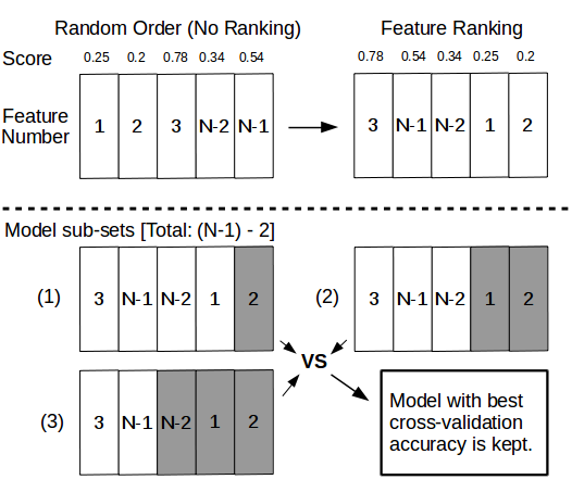
  Figure 13: Using scoring methods to rank features while training and testing. While datasets with N-1 features resulting from multiple reciprocal blastp alignments can be used to train and test machine learning models (see Figure 4), scoring functions can be applied to rank features and create model sub-sets that are in turn trained and tested in order to save the model sub-set with the highest classification accuracy.

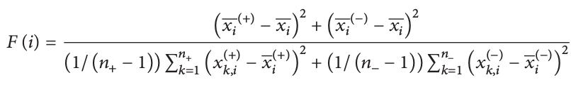
Figure 14: F score function. Given that our models contain N-1 binary features, we can use the F score function [4] to rank features based on their ability to tell a positive sample from a negative sample. x_i , x_i⁽⁺⁾, and x_i^(-) are the mean of the i_th feature of the total, positive, and negative samples respectively. x_k,i⁽⁺⁾ is the i_th feature of the k_th postive sample, while x_k,i^(-) is the i_th feature of the k_th negative sample.

• Model training.

  We mentioned earlier that data points of a training set are often expected to be linearly separable. However, this is not always the case. In order to properly separate datapoints, we can implement kernel functions with the purpose of mapping the original finite-dimensional space into a higher-dimensional space. We will be implementing a Gaussian kernel function in Sci-Kit Learn (a ML Library in Python).

• Model testing.

  We will be performing 10-fold cross-validation in order to test each one of our classification models.

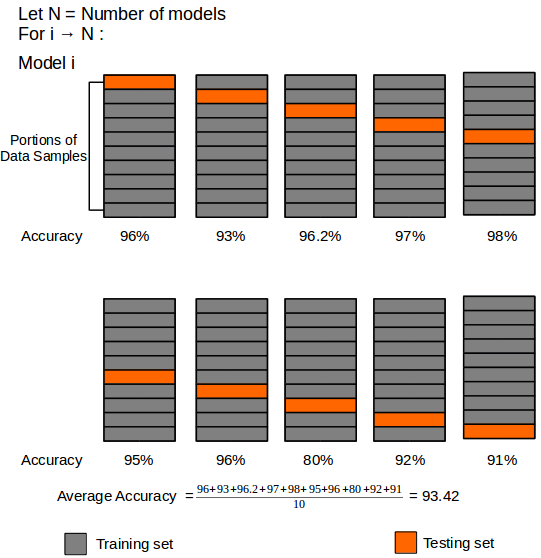
Figure 15: Schematic of 10-fold cross-validation. The training data is randomly sorted and divided into 10 equal portions, where 9 portions are used to train the classification model, and 1 portion is used as a testing set. The process is repeated until all portions are used as testing sets. 10-fold cross-validation follows the Pareto principle, which states that in most events at least 80% of the effects come from 20% of the causes.

All work will be carried out and monitored through the bioXJMB Slack group.

@bioXJMB

---

References:

[1] Hong-Li Hua, et al. (2016). An Approach for Predicting Essential Genes Using Multiple Homology Mapping and Machine Learning Algorithms. BioMed Research International. Volume 2016, Article ID 7639397.

[2] Qi Ji et al. (2003). Whole Proteome Prokaryote Phylogeny Without Sequence Alignment: A K-String Composition Approach. J Mol Evol. 58:1–11.

[3] Brendel V, et al. (1986) Linguistics of nucleotide sequences: Morphology and comparison of vocabularies. J Biomol Struct Dyn 4:11–21

[4] Y.-W. Chen & C.-J Lin. (2006). Combining SVMs with various feature selection strategies. Studies in Fuzziness and Soft Computing. 207:315–324.

Project Coordinator:

• Charles Sanfiorenzo - csanfior@caltech.edu